4-2最佳实践

本文参考：

• NVIDIA CUDA C best practice

概述

介绍

The CUDA C++ Best Practices Guide provides practical guidelines for writing high-performance CUDA applications. It covers optimization strategies across memory usage, parallel execution, and instruction-level efficiency. The guide helps developers identify performance bottlenecks, leverage GPU architecture effectively, and apply profiling tools to fine-tune applications. It’s an essential resource for maximizing throughput and achieving scalable, efficient CUDA programs.

本最佳实践指南是一本帮助开发者从 NVIDIA® CUDA® GPU 获得最佳性能的手册。它介绍了成熟的并行化和优化技术，并阐释了能极大简化支持 CUDA 的 GPU 架构编程工作的编码隐喻和惯用法。

虽然本指南的内容可用作参考手册，但需要注意的是，随着对各种编程和配置主题的探讨，有些主题会在不同情境下被重新提及。因此，建议初次阅读的读者按顺序阅读本指南。这种方式将极大加深您对高效编程实践的理解，并使您日后能更好地将本指南用作参考工具。

需求：

• CUDA Installation Guide
• CUDA C++ Programming Guide
• CUDA Toolkit Reference Manual

APOD 方法

This guide introduces the Assess, Parallelize, Optimize, Deploy(APOD) design cycle for applications with the goal of helping application developers to rapidly identify the portions of their code that would most readily benefit from GPU acceleration, rapidly realize that benefit, and begin leveraging the resulting speedups in production as early as possible.

APOD 是一个循环过程：只需投入最少的初始时间，就能实现、测试并部署初始的速度提升，此时可以通过识别更多优化机会、获得额外的速度提升，然后将更快版本的应用程序部署到生产环境中，从而再次开始这个循环。

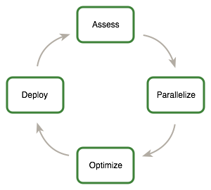
• Assess
  • For an existing project, the first step is to assess the application to locate the parts of the code that are responsible for the bulk of the execution time. Armed with this knowledge, the developer can evaluate these bottlenecks for parallelization and start to investigate GPU acceleration.By understanding the end-user’s requirements and constraints and by applying Amdahl’s and Gustafson’s laws, the developer can determine the upper bound of performance improvement from acceleration of the identified portions of the application.
• Parallelize
  • Having identified the hotspots and having done the basic exercises to set goals and expectations, the developer needs to parallelize the code.
• Optimize
  • After each round of application parallelization is complete, the developer can move to optimizing the implementation to improve performance. Since there are many possible optimizations that can be considered, having a good understanding of the needs of the application can help to make the process as smooth as possible. It is not necessary for a programmer to spend large amounts of time memorizing the bulk of all possible optimization strategies prior to seeing good speedups. Instead, strategies can be applied incrementally as they are learned.
  • Optimizations can be applied at various levels, from overlapping data transfers with computation all the way down to fine-tuning floating-point operation sequences. The available profiling tools are invaluable for guiding this process, as they can help suggest a next-best course of action for the developer’s optimization efforts and provide references into the relevant portions of the optimization section of this guide.
• Deploy
  • Having completed the GPU acceleration of one or more components of the application it is possible to compare the outcome with the original expectation. Recall that the initial assess step allowed the developer to determine an upper bound for the potential speedup attainable by accelerating given hotspots.

本指南给出了根据效果和使用范围确定的不同优先级的建议，需要优先考虑高优先级的建议。

错误检查

Code samples throughout the guide omit error checking for conciseness. Production code should, however, systematically check the error code returned by each API call and check for failures in kernel launches by calling cudaGetLastError().

回顾 CUDA 异构编程

CUDA programming involves running code on two different platforms concurrently: a host system with one or more CPUs and one or more CUDA-enabled NVIDIA GPU devices.

Differences between Host and Device

• Threading resources
  • Execution pipelines on host systems can support a limited number of concurrent threads. By comparison, the smallest executable unit of parallelism on a CUDA device comprises 32 threads (termed a warp of threads).
• Threads
  • Threads on a CPU are generally heavyweight entities. The operating system must swap threads on and off CPU execution channels to provide multithreading capability. Context switches (when two threads are swapped) are therefore slow and expensive. By comparison, threads on GPUs are extremely lightweight. In a typical system, thousands of threads are queued up for work (in warps of 32 threads each). If the GPU must wait on one warp of threads, it simply begins executing work on another. Because separate registers are allocated to all active threads, no swapping of registers or other state need occur when switching among GPU threads. Resources stay allocated to each thread until it completes its execution. In short, CPU cores are designed to minimize latency for a small number of threads at a time each, whereas GPUs are designed to handle a large number of concurrent, lightweight threads in order to maximize throughput.
• RAM
  • The host system and the device each have their own distinct attached physical memories 1. As the host and device memories are separated, items in the host memory must occasionally be communicated between device memory and host memory as described in What Runs on a CUDA-Enabled Device?.

1On Systems on a Chip with integrated GPUs, such as NVIDIA® Tegra®, host and device memory are physically the same, but there is still a logical distinction between host and device memory. See the Application Note on CUDA for Tegra for details.

What runs on a CUDA-enabled device?

• The device is ideally suited for computations that can be run on numerous data elements simultaneously in parallel.
• To use CUDA, data values must be transferred from the host to the device. These transfers are costly in terms of performance and should be minimized. (See Data Transfer Between Host and Device.) This cost has several ramifications:
  • The complexity of operations should justify the cost of moving data to and from the device.
  • Data should be kept on the device as long as possible. Because transfers should be minimized, programs that run multiple kernels on the same data should favor leaving the data on the device between kernel calls, rather than transferring intermediate results to the host and then sending them back to the device for subsequent calculations.Data Transfer Between Host and Device provides further details, including the measurements of bandwidth between the host and the device versus within the device proper.
• For best performance, there should be some coherence in memory access by adjacent threads running on the device. Certain memory access patterns enable the hardware to coalesce groups of reads or writes of multiple data items into one operation. Data that cannot be laid out so as to enable coalescing, or that doesn’t have enough locality to use the L1 or texture caches effectively, will tend to see lesser speedups when used in computations on GPUs.

Host and Device

CPU 是最小延迟的轻量并发架构，GPU 是最大吞吐的高并发架构。二者有独立内存，需要平衡“计算与数据传输”。

---

Profile

There are many possible approaches to profiling the code, but in all cases the objective is the same: to identify the function or functions in which the application is spending most of its execution time.

High Priority: To maximize developer productivity, profile the application to determine hotspots and bottlenecks.

The most important consideration with any profiling activity is to ensure that the workload is realistic.

CPU 的性能分析工具有 perf/gprof 等等

Understanding Scaling

The amount of performance benefit an application will realize by running on CUDA depends entirely on the extent to which it can be parallelized. Code that cannot be sufficiently parallelized should run on the host, unless doing so would result in excessive transfers between the host and the device.

High Priority: To get the maximum benefit from CUDA, focus first on finding ways to parallelize sequential code.

By understanding how applications can scale it is possible to set expectations and plan an incremental parallelization strategy. Strong Scaling and Amdahl’s Law describes strong scaling, which allows us to set an upper bound for the speedup with a fixed problem size. Weak Scaling and Gustafson’s Law describes weak scaling, where the speedup is attained by growing the problem size. In many applications, a combination of strong and weak scaling is desirable.

Strong Scaling and Amdahl’s Law

Strong scaling is a measure of how, for a fixed overall problem size, the time to solution decreases as more processors are added to a system. An application that exhibits linear strong scaling has a speedup equal to the number of processors used.

Strong scaling is usually equated with Amdahl’s Law, which specifies the maximum speedup that can be expected by parallelizing portions of a serial program. Essentially, it states that the maximum speedup S of a program is:

$$S=\frac{1}{(1-P)+P/N}$$

Here P is the fraction of the total serial execution time taken by the portion of code that can be parallelized and N is the number of processors over which the parallel portion of the code runs.

The larger N is(that is, the greater the number of processors), the smaller the P/N fraction. It can be simpler to view N as a very large number, which essentially transforms the equation into$S=1/(1-P)$. Now, if 3/4 of the running time of a sequential program is parallelized, the maximum speedup over serial code is 1 / (1 - 3/4) = 4.

In reality, most applications do not exhibit perfectly linear strong scaling, even if they do exhibit some degree of strong scaling. For most purposes, the key point is that the larger the parallelizable portion P is, the greater the potential speedup. Conversely, if P is a small number (meaning that the application is not substantially parallelizable), increasing the number of processors N does little to improve performance. Therefore, to get the largest speedup for a fixed problem size, it is worthwhile to spend effort on increasing P, maximizing the amount of code that can be parallelized.

Weak Scaling and Gustafson’s Law

Weak scaling is a measure of how the time to solution changes as more processors are added to a system with a fixed problem size per processor; i.e., where the overall problem size increases as the number of processors is increased.

Weak scaling is often equated with Gustafson’s Law, which states that in practice, the problem size scales with the number of processors. Because of this, the maximum speedup S of a program is:

$$S=N+(1-P)(1-N)$$

Here P is the fraction of the total serial execution time taken by the portion of code that can be parallelized and N is the number of processors over which the parallel portion of the code runs.

Another way of looking at Gustafson’s Law is that it is not the problem size that remains constant as we scale up the system but rather the execution time. Note that Gustafson’s Law assumes that the ratio of serial to parallel execution remains constant, reflecting additional cost in setting up and handling the larger problem.

强扩展的本质是问题总大小不变（比如计算 100 万组数据），通过增加处理器数量，减少“完成计算的总时间”。

• 阿姆达尔定律量化了强扩展的最大速度提升（S），核心逻辑是“程序总有无法并行的串行部分，这部分会限制整体提速”
• 强扩展的优化重点是最大化 P（增加可并行代码的比例），而非单纯加处理器。 弱扩展的本质是每个处理器的任务量不变，通过增加处理器数量，同步扩大“整体问题规模”，目标是让“总计算时间基本不变”。
• 古斯塔夫森定律的核心假设是“执行时间基本不变”，通过扩大问题规模，让“可并行部分的收益”覆盖“串行部分的固定开销”（比如多处理器的通信、任务分配等额外成本）。
• 弱扩展更适合“问题规模可灵活调整”的场景（比如大数据分析、科学计算），此时增加处理器的收益更明显。

Getting Thre Right Answer

• A key aspect of correctness verification for modifications to any existing program is to establish some mechanism whereby previous known-good reference outputs from representative inputs can be compared to new results.
• Unit test: A useful counterpart to the reference comparisons described above is to structure the code itself in such a way that is readily verifiable at the unit level.
  • Going a step further, if most functions are defined as __host__ __device__ rather than just __device__ functions, then these functions can be tested on both the CPU and the GPU, thereby increasing our confidence that the function is correct and that there will not be any unexpected differences in the results. If there are differences, then those differences will be seen early and can be understood in the context of a simple function.
• Debugging
  • CUDA-GDB is a port of the GNU Debugger that runs on Linux and Mac; see: https://developer.nvidia.com/cuda-gdb.
  • The NVIDIA Nsight Visual Studio Edition is available as a free plugin for Microsoft Visual Studio; see: https://developer.nvidia.com/nsight-visual-studio-edition.
  • Several third-party debuggers support CUDA debugging as well; see: https://developer.nvidia.com/debugging-solutions for more details.
• Numerical Accuracy and Precision
  • Incorrect or unexpected results arise principally from issues of floating-point accuracy due to the way floating-point values are computed and stored. See also https://developer.nvidia.com/content/precision-performance-floating-point-and-ieee-754-compliance-nvidia-gpus.
  • Single vs. Double Precision. Double Precision Results obtained using double-precision arithmetic will frequently differ from the same operation performed via single-precision arithmetic due to the greater precision of the former and due to rounding issues.
  • Floating Point Math Is Not Associative. This limitation is not specific to CUDA, but an inherent part of parallel computation on floating-point values.
  • IEEE 754 Compliance. All CUDA compute devices follow the IEEE 754 standard for binary floating-point representation, with some small exceptions. These exceptions, which are detailed in Features and Technical Specifications of the CUDA C++ Programming Guide, can lead to results that differ from IEEE 754 values computed on the host system.
  • One of the key differences is the fused multiply-add (FMA) instruction, which combines multiply-add operations into a single instruction execution. Its result will often differ slightly from results obtained by doing the two operations separately.
  • x86 80-bit Computations: x86 processors can use an 80-bit double extended precision math when performing floating-point calculations. The results of these calculations can frequently differ from pure 64-bit operations performed on the CUDA device.

数值精度和准确性会是计算验证的主要问题。

---

Performance Metrics

Timing

Using CPU Timers

Any CPU timer can be used to measure the elapsed time of a CUDA call or kernel execution.

• When using CPU timers, it is critical to remember that many CUDA API functions are asynchronous; that is, they return control back to the calling CPU thread prior to completing their work.
• Although it is also possible to synchronize the CPU thread with a particular stream or event on the GPU, these synchronization functions are not suitable for timing code in streams other than the default stream.

大多 CUDA API 是异步执行，要准确测量某个特定 CUDA 调用或某组 CUDA 调用序列的耗时，计时开始和结束需要同步。 使用流同步只能使用默认流。

Using CUDA GPU Timers

The CUDA event API provides calls that create and destroy events, record events (including a timestamp), and convert timestamp differences into a floating-point value in milliseconds. How to time code using CUDA events illustrates their use.

• How to time code using CUDA events:

cudaEvent_t start, stop;
float time;
 
cudaEventCreate(&start);
cudaEventCreate(&stop);
 
cudaEventRecord( start, 0 );
kernel<<<grid,threads>>> ( d_odata, d_idata, size_x, size_y,
                           NUM_REPS);
cudaEventRecord( stop, 0 );
cudaEventSynchronize( stop );
 
cudaEventElapsedTime( &time, start, stop );
cudaEventDestroy( start );
cudaEventDestroy( stop );

Here cudaEventRecord() is used to place the start and stop events into the default stream, stream 0. The device will record a timestamp for the event when it reaches that event in the stream. The cudaEventElapsedTime() function returns the time elapsed between the recording of the start and stop events. This value is expressed in milliseconds and has a resolution of approximately half a microsecond. Like the other calls in this listing, their specific operation, parameters, and return values are described in the CUDA Toolkit Reference Manual. Note that the timings are measured on the GPU clock, so the timing resolution is operating-system-independent.

CUDA 提供专门的事件 API（Event API） 实现 GPU 端计时，直接基于 GPU 时钟，精度更高（约 0.5 微秒）且不受操作系统影响，核心逻辑是“在 GPU 流中插入‘开始/结束’事件，计算两事件的时间差”。

注意本节所述的 CPU 与 GPU 同步点（如各类同步函数）会导致 GPU 处理流水线出现停滞（stall），因此要谨慎使用同步以减少其对性能的影响。

Bandwidth

Bandwidth - the rate at which data can be transferred - is one of the most important gating factors for performance. Almost all changes to code should be made in the context of how they affect bandwidth. As described in Memory Optimizations of this guide, bandwidth can be dramatically affected by the choice of memory in which data is stored, how the data is laid out and the order in which it is accessed, as well as other factors.

High Priority: Use the effective bandwidth of your computation as a metric when measuring performance and optimization benefits.

Theoretical Bandwidth Calculation

Theoretical bandwidth can be calculated using hardware specifications available in the product literature. For example, the NVIDIA Tesla V100 uses HBM2 (double data rate) RAM with a memory clock rate of 877 MHz and a 4096-bit-wide memory interface.

Using these data items, the peak theoretical memory bandwidth of the NVIDIA Tesla V100 is 898 GB/s:

$(0.877\times 10^9\times (4096/8)\times 2)÷10^9=898\text{GB/s}$

In this calculation, the memory clock rate is converted in to Hz, multiplied by the interface width (divided by 8, to convert bits to bytes) and multiplied by 2 due to the double data rate. Finally, this product is divided by 109 to convert the result to GB/s.

Effective Bandwidth Calculation

Effective bandwidth is calculated by timing specific program activities and by knowing how data is accessed by the program. To do so, use this equation:

$$effectivebandwidt=((B_r+B_w)/10^9)/time$$

Here, the effective bandwidth is in units of $GB/s$, $Br$ is the number of bytes read per kernel, $Bw$ is the number of bytes written per kernel, and time is given in seconds.

Throughput Reported by Visual Profiler

For devices with compute capability of 2.0 or greater, the Visual Profiler can be used to collect several different memory throughput measures. The following throughput metrics can be displayed in the Details or Detail Graphs view:

• Requested Global Load Throughput
• Requested Global Store Throughput
• Global Load Throughput
• Global Store Throughput
• DRAM Read Throughput
• DRAM Write Throughput

The Requested Global Load Throughput and Requested Global Store Throughput values indicate the global memory throughput requested by the kernel and therefore correspond to the effective bandwidth obtained by the calculation shown under Effective Bandwidth Calculation.

Because the minimum memory transaction size is larger than most word sizes, the actual memory throughput required for a kernel can include the transfer of data not used by the kernel. For global memory accesses, this actual throughput is reported by the Global Load Throughput and Global Store Throughput values.

It’s important to note that both numbers are useful. The actual memory throughput shows how close the code is to the hardware limit, and a comparison of the effective or requested bandwidth to the actual bandwidth presents a good estimate of how much bandwidth is wasted by suboptimal coalescing of memory accesses (see Coalesced Access to Global Memory). For global memory accesses, this comparison of requested memory bandwidth to actual memory bandwidth is reported by the Global Memory Load Efficiency and Global Memory Store Efficiency metrics.

带宽

1. 理论带宽通过硬件规模计算。
2. 有效带宽根据读取的数据量和实际耗时计算。
3. 吞吐量报告可显示：
4. “请求全局加载/存储吞吐量”对应“有效带宽计算”结果，反映内核请求的全局内存吞吐量。
5. “全局加载/存储吞吐量”反映实际内存吞吐量（因内存最小事务大小大于多数字长，可能包含程序未使用的数据传输）。
6. 二者对比可估计带宽浪费。

---

Memory Optimizations

Execution Configuration Optimizations

Instruction Optimization

---

硬件环境与部署

Deploying CUDA Applications

15. Understanding the Programming Environment

16. CUDA Compatibility Developer’s Guide

17. Preparing for Deployment

18. Deployment Infrastructure Tools