Summary Slides see also CompanionAsset_9780128119051.
Ch3 Instruction-level Parallelism and Its Exploitation
Instruction-Level Parallelism
- Pipelining become universal technique in 1985
- Overlaps execution of instructions
- Exploits “Instruction Level Parallelism”
- Beyond this, there are two main approaches:
- Hardware-based dynamic approaches
- Used in server and desktop processors
- Not used as extensively in PMP processors
- Compiler-based static approaches
- Not as successful outside of scientific applications
- Hardware-based dynamic approaches
- When exploiting instruction-level parallelism, goal is to maximize CPI
Pipeline CPI = Ideal pipeline CPI +Structural stalls +Data hazard stalls +Control stalls
- Parallelism with basic block is limited
- Typical size of basic block = 3-6 instructions
- Must optimize across branches
Dependence
- Loop-Level Parallelism
- Unroll loop statically or dynamically
- Use SIMD (vector processors and GPUs)
- Challenges:
- Data dependency
- Instruction j is data dependent on instruction i if
- Instruction i produces a result that may be used by instruction j
- Instruction j is data dependent on instruction k and instruction k is data dependent on instruction i
- Instruction j is data dependent on instruction i if
- Data dependency
- Dependent instructions cannot be executed simultaneously
- Dependencies are a property of programs
- Pipeline organization determines if dependence is detected and if it causes a stall
- Data dependence conveys:
- Possibility of a hazard
- Order in which results must be calculated
- Upper bound on exploitable instruction level parallelism
- Dependencies that flow through memory locations are difficult to detect
- Name Dependence: Two instructions use the same name but no flow of information
- Not a true data dependence, but is a problem when reordering instructions
- Antidependence: instruction j writes a register or memory location that instruction i reads
- Initial ordering (i before j) must be preserved
- Output dependence: instruction i and instruction j write the same register or memory location
- Ordering must be preserved
- To resolve, use register renaming techniques
- Data Hazards
- Read after write (RAW)
- Write after write (WAW)
- Write after read (WAR)
- Control Dependence
- Ordering of instruction i with respect to a branch instruction
- Instruction control dependent on a branch cannot be moved before the branch so that its execution is no longer controlled by the branch
- An instruction not control dependent on a branch cannot be moved after the branch so that its execution is controlled by the branch
- Ordering of instruction i with respect to a branch instruction
Compiler Techniques for Exposing ILP
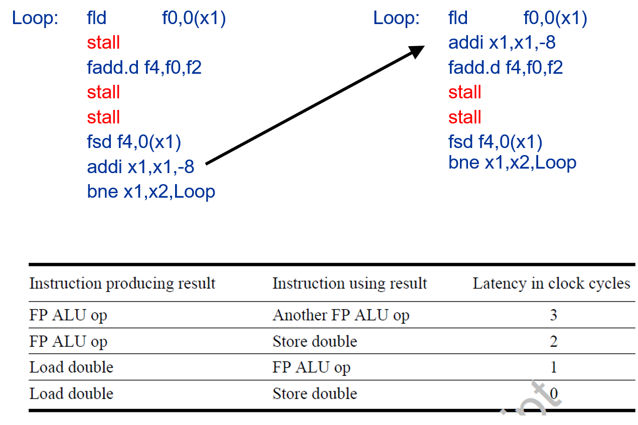
- Pipeline scheduling
- Separate dependent instruction from the source instruction by the pipeline latency of the source instruction
- Example:
for (i=999; i>=0; i=i-1) x[i] = x[i] + s;
- Loop Unrolling
- Unroll by a factor of 4 (assume # elements is divisible by 4)
- Eliminate unnecessary instructions
- Strip Mining
- Unknown number of loop iterations?
- Number of iterations = n
- Goal: make k copies of the loop body
- Generate pair of loops:
- First executes n mod k times
- Second executes n / k times
- “Strip mining”
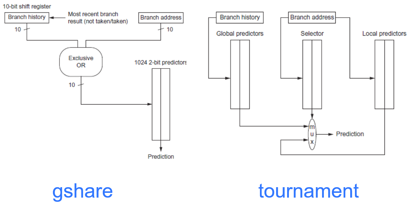
Branch Prediction
- Basic 2-bit predictor:
- For each branch:
- Predict taken or not taken
- If the prediction is wrong two consecutive times, change prediction
- For each branch:
- Correlating predictor:
- Multiple 2-bit predictors for each branch
- One for each possible combination of outcomes of preceding n branches
- (m, n) predictor: behavior from last m branches to choose from 2m n-bit predictors
- Tournament predictor:
- Combine correlating predictor with local predictor
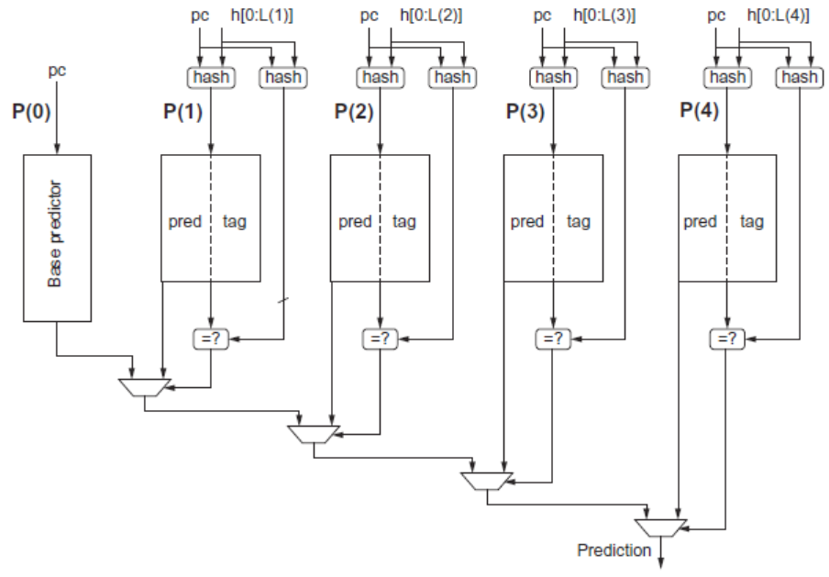
- Tagged Hybrid Predictors
- Need to have predictor for each branch and history
- Problem: this implies huge tables
- Solution:
- Use hash tables, whose hash value is based on branch address and branch history
- Longer histories may lead to increased chance of hash collision, so use multiple tables with increasingly shorter histories
 See Also https://github.com/sjdesai16/tage.
Dynamic Scheduling
- Rearrange order of instructions to reduce stalls while maintaining data flow
- Advantages:
- Compiler doesn’t need to have knowledge of microarchitecture
- Handles cases where dependencies are unknown at compile time
- Disadvantage:
- Substantial increase in hardware complexity
- Complicates exceptions
- Advantages:
- Dynamic scheduling implies:
- Out-of-order execution
- Out-of-order completion
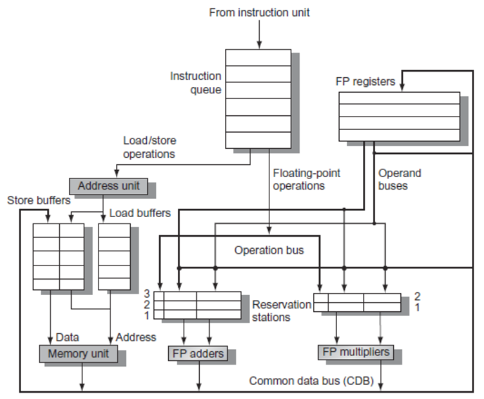
Register Renaming
- Tomasulo’s Approach
- Tracks when operands are available
- Introduces register renaming in hardware
- Minimizes WAW and WAR hazards
- Register renaming is provided by reservation stations (RS)
- Contains:
- The instruction
- Buffered operand values (when available)
- Reservation station number of instruction providing the operand values
- Contains:
- RS fetches and buffers an operand as soon as it becomes available (not necessarily involving register file)
- Pending instructions designate the RS to which they will send their output
- Result values broadcast on a result bus, called the common data bus (CDB)
- Only the last output updates the register file
- As instructions are issued, the register specifiers are renamed with the reservation station
- May be more reservation stations than registers
- Load and store buffers
- Contain data and addresses, act like reservation stations
- Three Steps:
- Issue
- Get next instruction from FIFO queue
- If available RS, issue the instruction to the RS with operand values if available
- If operand values not available, stall the instruction
- Execute
- When operand becomes available, store it in any reservation stations waiting for it
- When all operands are ready, issue the instruction
- Loads and store maintained in program order through effective address
- No instruction allowed to initiate execution until all branches that proceed it in program order have completed
- Write result
- Write result on CDB into reservation stations and store buffers
- (Stores must wait until address and value are received)
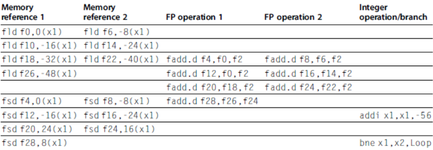
- Example loop:
Loop:  fld f0,0(x1)
  fmul.d f4,f0,f2
  fsd f4,0(x1)
  addi x1,x1,8
  bne x1,x2,Loop // branches if x16 != x2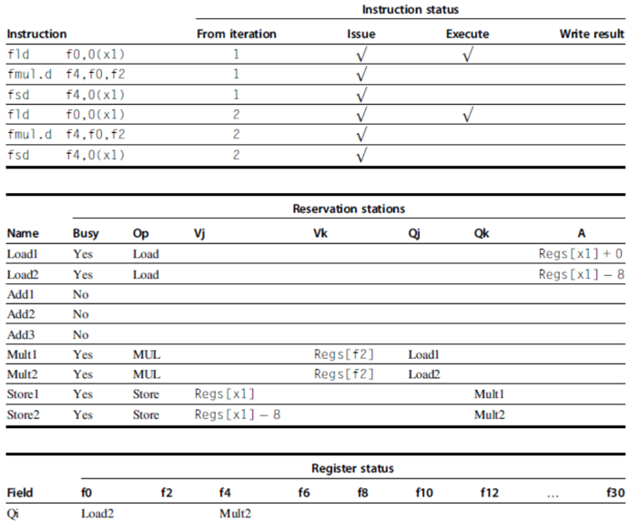
Hardware-Based Speculation
- Execute instructions along predicted execution paths but only commit the results if prediction was correct
- Instruction commit: allowing an instruction to update the register file when instruction is no longer speculative
- Need an additional piece of hardware to prevent any irrevocable action until an instruction commits
- I.e. updating state or taking an execution
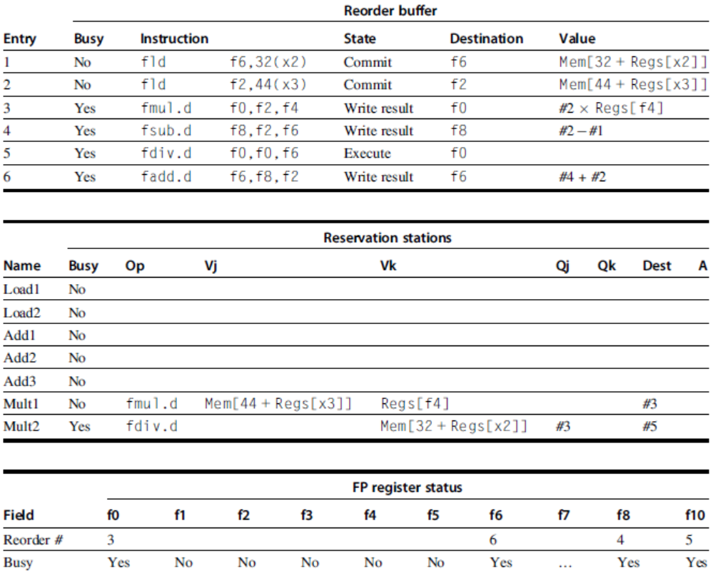
- Reorder buffer – holds the result of instruction between completion and commit
- Four fields:
- Instruction type: branch/store/register
- Destination field: register number
- Value field: output value
- Ready field: completed execution?
- Modify reservation stations:
- Operand source is now reorder buffer instead of functional unit
- Issue:
- Allocate RS and ROB, read available operands
- Execute:
- Begin execution when operand values are available
- Write result:
- Write result and ROB tag on CDB
- Commit:
- When ROB reaches head of ROB, update register
- When a mispredicted branch reaches head of ROB, discard all entries
- Register values and memory values are not written until an instruction commits
- On misprediction:
- Speculated entries in ROB are cleared
- Exceptions:
- Not recognized until it is ready to commit
- On misprediction:
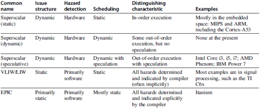
Multiple Issue and Static Scheduling
- To achieve CPI < 1, need to complete multiple instructions per clock
- Solutions:
- Statically scheduled superscalar processors
- VLIW (very long instruction word) processors
- Dynamically scheduled superscalar processors
- VLIW Processors
- Package multiple operations into one instruction
- Example VLIW processor:
- One integer instruction (or branch)
- Two independent floating-point operations
- Two independent memory references
- Must be enough parallelism in code to fill the available slots
- Disadvantages:
- Statically finding parallelism
- Code size
- No hazard detection hardware
- Binary code compatibility
- Modern microarchitectures: Dynamic scheduling + multiple issue + speculation
- Two approaches:
- Assign reservation stations and update pipeline control table in half clock cycles
- Only supports 2 instructions/clock
- Design logic to handle any possible dependencies between the instructions
- Assign reservation stations and update pipeline control table in half clock cycles
- Issue logic is the bottleneck in dynamically scheduled superscalars
- Multiple Issue
- Examine all the dependencies among the instructions in the bundle
- If dependencies exist in bundle, encode them in reservation stations
- Also need multiple completion/commit
- To simplify RS allocation:
- Limit the number of instructions of a given class that can be issued in a “bundle”, i.e. on FP, one integer, one load, one store
Loop:  ld x2,0(x1)  //x2=array element
  addi x2,x2,1  //increment x2
  sd x2,0(x1)  //store result
  addi x1,x1,8  //increment pointer
bne x2,x3,Loop //branch if not last.png)
.png)
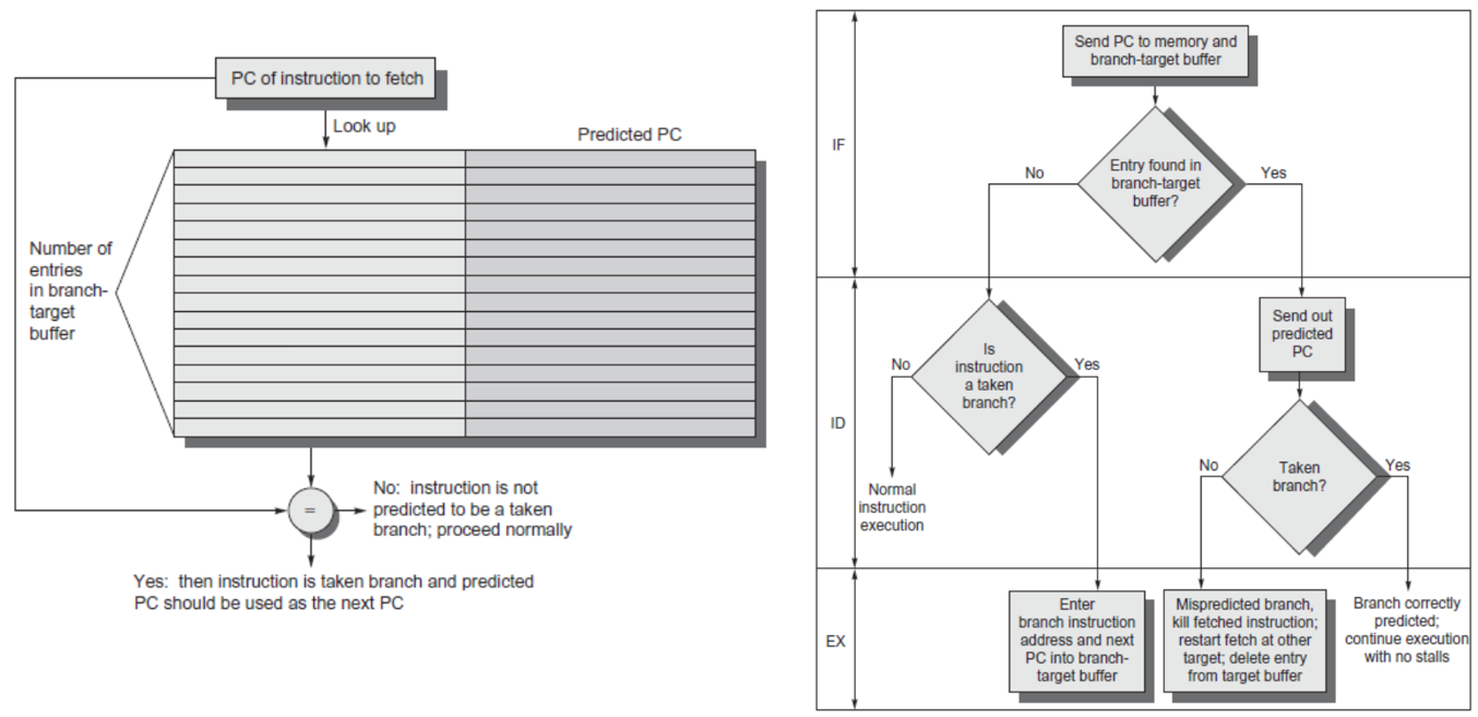
Branch -Target Buffer
- Need high instruction bandwidth
- Branch-Target buffers
- Next PC prediction buffer, indexed by current PC
- Branch-Target buffers
- Branch Folding
- Optimization:
- Larger branch-target buffer
- Add target instruction into buffer to deal with longer decoding time required by larger buffer
- “Branch folding”
- Return Address Predictor
- Most unconditional branches come from function returns
- The same procedure can be called from multiple sites
- Causes the buffer to potentially forget about the return address from previous calls
- Create return address buffer organized as a stack
Integrated Instruction Fetch Unit
- Design monolithic unit that performs:
- Branch prediction
- Instruction prefetch
- Fetch ahead
- Instruction memory access and buffering
- Deal with crossing cache lines
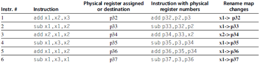
- Register renaming vs. reorder buffers
- Instead of virtual registers from reservation stations and reorder buffer, create a single register pool
- Contains visible registers and virtual registers
- Use hardware-based map to rename registers during issue
- WAW and WAR hazards are avoided
- Speculation recovery occurs by copying during commit
- Still need a ROB-like queue to update table in order
- Simplifies commit:
- Record that mapping between architectural register and physical register is no longer speculative
- Free up physical register used to hold older value
- In other words: SWAP physical registers on commit
- Physical register de-allocation is more difficult
- Simple approach: deallocate virtual register when next instruction writes to its mapped architecturally-visibly register
- Instead of virtual registers from reservation stations and reorder buffer, create a single register pool
- Combining instruction issue with register renaming:
- Issue logic pre-reserves enough physical registers for the bundle
- Issue logic finds dependencies within bundle, maps registers as necessary
- Issue logic finds dependencies between current bundle and already in-flight bundles, maps registers as necessary
- How much to speculate
- Mis-speculation degrades performance and power relative to no speculation
- May cause additional misses (cache, TLB)
- Prevent speculative code from causing higher costing misses (e.g. L2)
- Mis-speculation degrades performance and power relative to no speculation
- Speculating through multiple branches
- Complicates speculation recovery
- Speculation and energy efficiency
- Note: speculation is only energy efficient when it significantly improves performance
- Value prediction
- Uses:
- Loads that load from a constant pool
- Instruction that produces a value from a small set of values
- Uses:
- Not incorporated into modern processors
- Similar idea—address aliasing prediction—is used on some processors to determine if two stores or a load and a store reference the same address to allow for reordering
Fallacies and Pitfalls
- It is easy to predict the performance/energy efficiency of two different versions of the same ISA if we hold the technology constant
- Processors with lower CPIs / faster clock rates will also be faster
- Sometimes bigger and dumber is better
- And sometimes smarter is better than bigger and dumber
- Believing that there are large amounts of ILP available, if only we had the right techniques
Ch 4 Data-Level Parallelism in Vector, SIMD, and GPU Architectures
- SIMD architectures can exploit significant data-level parallelism for:
- Matrix-oriented scientific computing
- Media-oriented image and sound processors
- SIMD is more energy efficient than MIMD
- Only needs to fetch one instruction per data operation
- Makes SIMD attractive for personal mobile devices
- SIMD allows programmer to continue to think sequentially
SIMD Parallelism
- Vector architectures
- SIMD extensions
- Graphics Processor Units (GPUs)
- For x86 processors:
- Expect two additional cores per chip per year
- SIMD width to double every four years
- Potential speedup from SIMD to be twice that from MIMD!
Vector Architectures
- Basic idea:
- Read sets of data elements into “vector registers”
- Operate on those registers
- Disperse the results back into memory
- Registers are controlled by compiler
- Used to hide memory latency
- Leverage memory bandwidth
VMIPS
- Example architecture: RV64V
- Loosely based on Cray-1
- 32 62-bit vector registers
- Register file has 16 read ports and 8 write ports
- Vector functional units
- Fully pipelined
- Data and control hazards are detected
- Vector load-store unit
- Fully pipelined
- One word per clock cycle after initial latency
- Scalar registers
- 31 general-purpose registers
- 32 floating-point registers
Vector Execution Time
- Execution time depends on three factors:
- Length of operand vectors
- Structural hazards
- Data dependencies
- RV64V functional units consume one element per clock cycle
- Execution time is approximately the vector length
- Convey
- Set of vector instructions that could potentially execute together
Chimes
- Sequences with read-after-write dependency hazards placed in same convey via chaining
- Chaining
- Allows a vector operation to start as soon as the individual elements of its vector source operand become available
- Chime
- Unit of time to execute one convey
- m conveys executes in m chimes for vector length n
- For vector length of n, requires m x n clock cycles
vld  v0,x5  # Load vector X
vmul  v1,v0,f0    # Vector-scalar multiply
vld  v2,x6  # Load vector Y
vadd  v3,v1,v2  # Vector-vector add
vst  v3,x6  # Store the sum

Convoys:
1    vld    vmul
2    vld    vadd
3    vst
3 chimes, 2 FP ops per result, cycles per FLOP = 1.5
For 64 element vectors, requires 32 x 3 = 96 clock cycles
- Challenges
- Start up time
- Latency of vector functional unit
- Assume the same as Cray-1
- Floating-point add ⇒ 6 clock cycles
- Floating-point multiply ⇒ 7 clock cycles
- Floating-point divide ⇒ 20 clock cycles
- Vector load ⇒ 12 clock cycles
- Improvements:
-
1 element per clock cycle
- Non-64 wide vectors
- IF statements in vector code
- Memory system optimizations to support vector processors
- Multiple dimensional matrices
- Sparse matrices
- Programming a vector computer
-
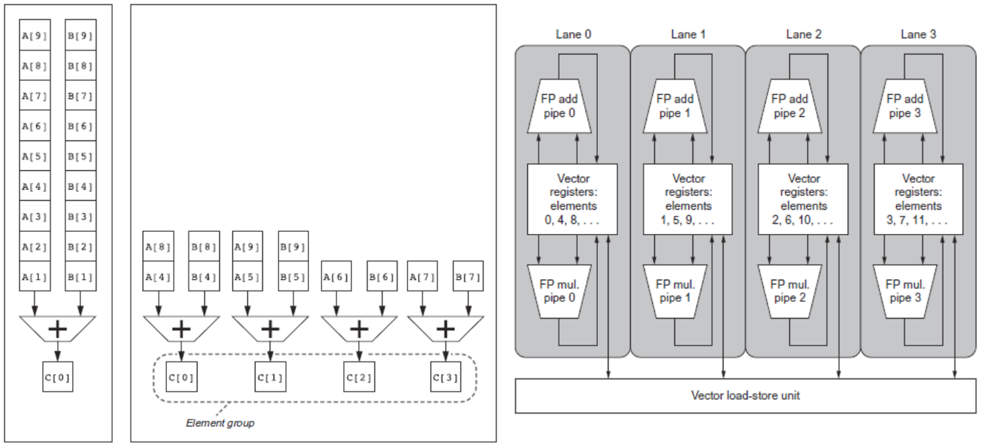
Multiple Lanes
- Element n of vector register A is “hardwired” to element n of vector register B
- Allows for multiple hardware lanes
- Consider:
  for (i = 0; i < 64; i=i+1)
	  if (X[i] != 0)
X[i] = X[i] – Y[i];- Use predicate register to “disable” elements:
Memory Banks
- Memory system must be designed to support high bandwidth for vector loads and stores
- Spread accesses across multiple banks
- Control bank addresses independently
- Load or store non sequential words (need independent bank addressing)
- Support multiple vector processors sharing the same memory
- Example:
- 32 processors, each generating 4 loads and 2 stores/cycle
- Processor cycle time is 2.167 ns, SRAM cycle time is 15 ns
- How many memory banks needed?
Stride
- Consider:
  for (i = 0; i < 100; i=i+1)
  	for (j = 0; j < 100; j=j+1) {
		  A[i][j] = 0.0;
		  for (k = 0; k < 100; k=k+1)
		  A[i][j] = A[i][j] + B[i][k] * D[k][j];
}- Must vectorize multiplication of rows of B with columns of D
- Use non-unit stride
- Bank conflict (stall) occurs when the same bank is hit faster than bank busy time:
Scatter-Gather
- Consider:
  for (i = 0; i < n; i=i+1)
A[K[i]] = A[K[i]] + C[M[i]];- Use index vector:
vsetdcfg  4*FP64  # 4 64b FP vector registers
vld  v0, x7  # Load K[]
vldx  v1, x5, v0  # Load A[K[]]
vld  v2, x28  # Load M[]
vldi  v3, x6, v2  # Load C[M[]]
vadd  v1, v1, v3  # Add them
vstx  v1, x5, v0  # Store A[K[]]
vdisable    # Disable vector registers
Programming Vec. Architectures
- Compilers can provide feedback to programmers
- Programmers can provide hints to compiler
SIMD Extensions
- Media applications operate on data types narrower than the native word size
- Example: disconnect carry chains to “partition” adder
- Limitations, compared to vector instructions:
- Number of data operands encoded into op code
- No sophisticated addressing modes (strided, scatter-gather)
- No mask registers
- Implementations:
- Intel MMX (1996)
- Eight 8-bit integer ops or four 16-bit integer ops
- Streaming SIMD Extensions (SSE) (1999)
- Eight 16-bit integer ops
- Four 32-bit integer/fp ops or two 64-bit integer/fp ops
- Advanced Vector Extensions (2010)
- Four 64-bit integer/fp ops
- AVX-512 (2017)
- Eight 64-bit integer/fp ops
- Operands must be consecutive and aligned memory locations
- Intel MMX (1996)
- Roofline Performance Model
- Basic idea:
- Plot peak floating-point throughput as a function of arithmetic intensity
- Ties together floating-point performance and memory performance for a target machine
- Arithmetic intensity
- Floating-point operations per byte read
- Examples: Attainable GFLOPs/sec = (Peak Memory BW × Arithmetic Intensity, Peak Floating Point Perf.)
- Basic idea:
Graphical Processing Units
- Basic idea:
- Heterogeneous execution model
- CPU is the host, GPU is the device
- Develop a C-like programming language for GPU
- Unify all forms of GPU parallelism as CUDA thread
- Programming model is “Single Instruction Multiple Thread”
- Heterogeneous execution model
- A thread is associated with each data element
- Threads are organized into blocks
- Blocks are organized into a grid
- GPU hardware handles thread management, not applications or OS
- NVIDIA GPU Architecture
- Similarities to vector machines:
- Works well with data-level parallel problems
- Scatter-gather transfers
- Mask registers
- Large register files
- Differences:
- No scalar processor
- Uses multithreading to hide memory latency
- Has many functional units, as opposed to a few deeply pipelined units like a vector processor
- Example
- Code that works over all elements is the grid
- Thread blocks break this down into manageable sizes
- 512 threads per block
- SIMD instruction executes 32 elements at a time
- Thus grid size = 16 blocks
- Block is analogous to a strip-mined vector loop with vector length of 32
- Block is assigned to a multithreaded SIMD processor by the thread block scheduler
- Current-generation GPUs have 7-15 multithreaded SIMD processors
- Terminology
- Each thread is limited to 64 registers
- Groups of 32 threads combined into a SIMD thread or “warp”
- Mapped to 16 physical lanes
- Up to 32 warps are scheduled on a single SIMD processor
- Each warp has its own PC
- Thread scheduler uses scoreboard to dispatch warps
- By definition, no data dependencies between warps
- Dispatch warps into pipeline, hide memory latency
- Thread block scheduler schedules blocks to SIMD processors
- Within each SIMD processor:
- 32 SIMD lanes
- Wide and shallow compared to vector processors
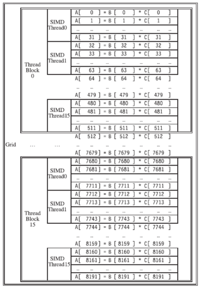
上图就是 Grid-Thread block-Thread 三级的数据工作分配示意图,是一个软件概念,实现了一个矩阵 - 向量乘。每个向量是 8192 个元素。每个 SIMD thread(warp)执行 32 个元素计算,每个 Thread block 包含 16 个 SIMD Thread,完成 512 个元素计算,Grid 包含 16 个 Thread block,完成整个 8192 个元素计算。Thread block 调度器将 16 个线程块分配到不同的 SM 上执行,只有一个 Thread block 内的 SIMD 线程可以通过 local memory 进行通信。
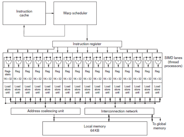
上图是 GPU 的 SM 组织形式图,可以直观看到 SM 中一个 warp 调度器将线程分配到 16 条 SIMD lane 上,一个 SM 中可能含有多个线程块。每个 lane 包含了 1024 个 32 位的寄存器,warp 调度器支持 32 条独立的 SIMD 线程指令,可以记录 32 条 PC。同一个线程块包含的 warp 可以通过 local memory 来通信。
NVIDIA Instruction Set Arch
- ISA is an abstraction of the hardware instruction set
- “Parallel Thread Execution (PTX)”
- opcode. type d, a, b, c;
- Uses virtual registers
- Translation to machine code is performed in software
- Example:
- “Parallel Thread Execution (PTX)”
shl.s32  R8, blockIdx, 9  ; Thread Block ID * Block size (512 or 29)
add.s32  R8, R8, threadIdx  ; R8 = i = my CUDA thread ID
ld.global.f64  RD0, [X+R8]  ; RD0 = X[i]
ld.global.f64  RD2, [Y+R8]  ; RD2 = Y[i]
mul.f64 R0D, RD0, RD4  ; Product in RD0 = RD0 * RD4 (scalar a)
add.f64 R0D, RD0, RD2  ; Sum in RD0 = RD0 + RD2 (Y[i])
st.global.f64 [Y+R8], RD0 ; Y[i] = sum (X[i]*a + Y[i])- Conditional Branching
- Like vector architectures, GPU branch hardware uses internal masks
- Also uses
- Branch synchronization stack
- Entries consist of masks for each SIMD lane
- I.e. which threads commit their results (all threads execute)
- Instruction markers to manage when a branch diverges into multiple execution paths
- Push on divergent branch
- …and when paths converge
- Act as barriers
- Pops stack
- Branch synchronization stack
- Per-thread-lane 1-bit predicate register, specified by programmer
- Example
  if (X[i] != 0)
	  X[i] = X[i] – Y[i];
  else X[i] = Z[i];

  ld.global.f64  RD0, [X+R8]  ; RD0 = X[i]
  setp.neq.s32  P1, RD0, #0  ; P1 is predicate register 1
  @!P1, bra  ELSE1, *Push  ; Push old mask, set new mask bits
					  ; if P1 false, go to ELSE1
  ld.global.f64  RD2, [Y+R8]  ; RD2 = Y[i]
  sub.f64  RD0, RD0, RD2  ; Difference in RD0
  st.global.f64  [X+R8], RD0  ; X[i] = RD0
  @P1, bra  ENDIF1, *Comp  ; complement mask bits
					  ; if P1 true, go to ENDIF1
ELSE1:  ld.global.f64 RD0, [Z+R8]  ; RD0 = Z[i]
  st.global.f64 [X+R8], RD0  ; X[i] = RD0
ENDIF1:   <next instruction>, *Pop  ; pop to restore old mask
NVIDIA GPU Memory Structures
- Each SIMD Lane has private section of off-chip DRAM
- “Private memory”
- Contains stack frame, spilling registers, and private variables
- Each multithreaded SIMD processor also has local memory
- Shared by SIMD lanes / threads within a block
- Memory shared by SIMD processors is GPU Memory
- Host can read and write GPU memory
Pascal Architecture Innovations
- Each SIMD processor has
- Two or four SIMD thread schedulers, two instruction dispatch units
- 16 SIMD lanes (SIMD width=32, chime=2 cycles), 16 load-store units, 4 special function units
- Two threads of SIMD instructions are scheduled every two clock cycles
- Fast single-, double-, and half-precision
- High Bandwidth Memory 2 (HBM2) at 732 GB/s
- NVLink between multiple GPUs (20 GB/s in each direction)
- Unified virtual memory and paging support
Vector Architectures Vs GPUs
- SIMD processor analogous to vector processor, both have MIMD
- Registers
- RV64V register file holds entire vectors
- GPU distributes vectors across the registers of SIMD lanes
- RV64 has 32 vector registers of 32 elements (1024)
- GPU has 256 registers with 32 elements each (8K)
- RV64 has 2 to 8 lanes with vector length of 32, chime is 4 to 16 cycles
- SIMD processor chime is 2 to 4 cycles
- GPU vectorized loop is grid
- All GPU loads are gather instructions and all GPU stores are scatter instructions
SIMD Architectures Vs GPUs
- GPUs have more SIMD lanes
- GPUs have hardware support for more threads
- Both have 2:1 ratio between doubleand single-precision performance
- Both have 64-bit addresses, but GPUs have smaller memory
- SIMD architectures have no scatter-gather support
Loop-Level Parallelism
- Focuses on determining whether data accesses in later iterations are dependent on data values produced in earlier iterations
- Loop-carried dependence
- Example 1:
  for (i=999; i>=0; i=i-1)
x[i] = x[i] + s;- No loop-carried dependence
- Example 2:
  for (i=0; i<100; i=i+1) {
	  A[i+1] = A[i] + C[i]; /* S1 */
	  B[i+1] = B[i] + A[i+1]; /* S2 */
}- S1 and S2 use values computed by S1 in previous iteration
- S2 uses value computed by S1 in same iteration
- Example 3:
  for (i=0; i<100; i=i+1) {
	  A[i] = A[i] + B[i]; /* S1 */
	  B[i+1] = C[i] + D[i]; /* S2 */
}- S1 uses value computed by S2 in previous iteration but dependence is not circular so loop is parallel
- Transform to:
	  A[0] = A[0] + B[0];
  for (i=0; i<99; i=i+1) {
	  B[i+1] = C[i] + D[i];
	  A[i+1] = A[i+1] + B[i+1];
  }
B[100] = C[99] + D[99];- Example 4:
  for (i=0;i<100;i=i+1)  {
	  A[i] = B[i] + C[i];
	  D[i] = A[i] * E[i];
} - Example 4:
  for (i=0;i<100;i=i+1)  {
	  A[i] = B[i] + C[i];
	  D[i] = A[i] * E[i];
}- Example 5:
  for (i=1;i<100;i=i+1)  {
	  Y[i] = Y[i-1] + Y[i];
  }
Finding Dependencies
- Assume indices are affine:
- (i is loop index)
- Assume:
- Store to a x i + b, then
- Load from c x i + d
- i runs from m to n
- Dependence exists if:
- Given j, k such that m ≤ j ≤ n, m ≤ k ≤ n
- Store to a x j + b, load from a x k + d, and a x j + b = c x k + d
- Generally cannot determine at compile time
- Test for absence of a dependence:
- GCD test:
- If a dependency exists, GCD (c, a) must evenly divide (d-b)
- GCD test:
Example:
for (i=0; i<100; i=i+1) {
  X[2*i+3] = X[2*i] * 5.0;
}
Example 2:
for (i=0; i<100; i=i+1) {
Y[i] = X[i] / c; /* S1 */
X[i] = X[i] + c; /* S2 */
Z[i] = Y[i] + c; /* S3 */
Y[i] = c - Y[i]; /* S4 */
}- Watch for antidependencies and output dependencies
Fallacies and Pitfalls
- GPUs suffer from being coprocessors
- GPUs have flexibility to change ISA
- Concentrating on peak performance in vector architectures and ignoring start-up overhead
- Overheads require long vector lengths to achieve speedup
- Increasing vector performance without comparable increases in scalar performance
- You can get good vector performance without providing memory bandwidth
- On GPUs, just add more threads if you don’t have enough memory performance